Page notes for Cartoon Climate, Revised Edition (2022)

Below please find page notes for The Cartoon Introduction to Climate Change, Revised Edition (2022). Note that occasional Wikipedia references are for topics that can be found in many introductory textbooks. References to IPCC AR6 Working Group 1 (“The Physical Science Basis”, 2021) are simply identified as AR6; references to earlier Assessment Reports are identified with a date, e.g., “AR5 (2014)”. 

Chapter 1: Introduction (pages 3-14)

Page 4, “Story #1 is about economic growth”: Just look at China! Also, an interesting read here is Bill Gates’s take-down of the myth that “poor countries are doomed to stay poor”.

Page 4, the invisible hand: The “invisible hand” idea is that individual self-interest can (“as if led by an invisible hand”) lead to economic growth and otherwise promote the common good. The metaphor comes from The Wealth of Nations (1776) by Adam Smith, who was a Scottish philosopher and “the father of modern economics”. For more on this see our Cartoon Econ books, especially Volume One: Microeconomics.

Page 5, world population: See UN World Population Prospects 2019, which projects 10.9 billion people in 2021 and has this graph; see also Pew. But see also this Lancet article from 2020, cited in the Guardian, which projects a peak of 9.7 billion in 2064.  

Page 5, “a world of 2-6 billion”: This refers to an article by a demographer in Journal of the Royal Statistical Society: Lutz 2009, “Towards a world of 2-6 billion well-educated and therefore healthy and wealthy people”.

Page 8, “pandemics”: Just taking a moment to pat ourselves on the back and note that the 1st edition (published in 2014, well before Covid) had something similar: “bird flu”.

Page 9, “alien planet”: This is an allusion to Harvard economist Marty Weitzman: “Societies and ecosystems whose average temperature has changed in the course of a century or so by T > 6°C (for U.S. readers: 6°C ≈11°F) are located in the terra incognita of what any honest economic modeler would have to admit is a planet Earth reconfigured as science fiction, since such high temperatures have not existed for some tens of millions of years.” From Weitzman 2007, “A Review of The Stern Review on the Economics of Climate Change“, Journal of Economic Literature 45:703-724.

Page 9, “wicked problem”: Believe it or not, “wicked problem” is a technical term. So is “super wicked problem”!

Page 12, “Seattle in July”: Thanks to Washington State’s Assistant State Climatologist Karin Bumbaco for helping out here; the temperature range given is based on the mean Seattle Sandpoint July temperature +/- one standard deviation over the period of record. On flowers blooming earlier, see Observed Changes in Phenology Across the United States – Pacific Northwest: “Across the Northwestern and interior Western U.S. time of first bloom for lilac (Syringa vulgaris) and honeysuckle (Lonicera tatarica and L. korolkowii) showed a trend toward earlier flowering (average advances of 7.5 days for lilac and 10 for honeysuckle) over an almost 40-year period.”

Page 12, “climate is like your personality, weather is like your mood”: There are other, similar comparisons, e.g., “climate is what you expect, weather is what you get” and “Climate tells you what clothes to buy, weather tells you what clothes to wear.” I’m not sure where the personality/mood comparison comes from, but I first came across it in a 2013 TEDx Atlanta talk by Marshall Shepherd, president of the American Meteorological Society, on “Slaying the ‘Zombies’ of Climate Science”.

Chapter 2: A brief history of Planet Earth (pages 15-26)

A good general reference for this chapter is David Catling’s Astrobiology: A Very Short Introduction (2014). Professor Catling also recommends these two books: Ruddiman’s Earth’s Climate: Past and Future (2nd ed., 2008) and (a bit more technical than Ruddiman’s) Kump, Kasting, and Crane’s The Earth System (3rd ed., 2009).

Page 15, “first the Earth cooled”: The line comes from the 1982 disaster spoof movie Airplane II: The Sequel:

Steve McCroskey: Jacobs, I want to know absolutely everything that’s happened up till now.

Jacobs: Well, let’s see. First the Earth cooled. And then the dinosaurs came, but they got too big and fat, so they all died and they turned into oil. And then the Arabs came and they bought Mercedes Benzes!

The sequel received mediocre reviews, but the original movie from 1980, called Airplane!, is regarded as surely one of the funniest movies of all time. (And don’t call me Shirley!)

Page 17, photosynthesis: More here. Note that not all photosynthesis is done by green things; for example there’s brown algae, such as kelp, red algae, etc.

Page 18, carbon cycle: See AR6 Figure 5.12, which shows “ocean-atmosphere gas exchange” of about 80 PgC and “gross photosynthesis” and “total respiration and fire” both at about 120 PgC. (Note that this graphic shows petagrams of carbon per year [PgC]; one petagram is 1 billion metric tons: 1 Pg = 10^15 grams = 10^12 kilograms = 10^9 metric tons; as NOAA puts it, a coal train containing 1 PgC would be about 156,000 miles long!) Older figures include AR5 (2014) Figure 6.1, this NASA graph, this more complicated figure from AR4 (2007) Figure 7.3, and this from NOAA.

Page 18, “mostly water and carbon”: By mass, the human body is about 53% water and 18% carbon. (We assume cows are similar.) Water seems to make up 50% or more of total plant weight, and in terms of dry-weight (i.e., besides the water) plants are about 50% carbon.

Page 19-21, ozone: Ozone exists in the atmosphere at two levels, both as the ozone layer (aka “stratospheric ozone” or “good ozone”), which occurs naturally in the layer of the upper atmosphere called the stratosphere, and as ground-level ozone (aka “troposheric ozone” or “bad ozone”) which contributes to smog and is mostly produced by cars and other human activities. More here on the ozone hole, which refers to the depletion of “good ozone” from the ozone layer.

Page 22, Snowball Earth and tropical North Pole: See more here about the Snowball Earth hypothesis. As for a tropical North Pole, see the Paleocene-Eocene Thermal Maximum (PETM) about 55 million years ago; see also “Studies Portray Tropical Arctic in Distant Past” (NY Times, June 1 2006).

Page 23, Carboniferous Period: See here, plus lots of other cool articles and images from the BBC, National Geographic, and the University of California Museum of Paleontology.

Page 24, continental drift: See this 2012 NPR story. Continental drift (and fingernails) grow at about 1 inch per year.

Page 24, “species either died off or slowly evolved into the forms they have today”: Professor Catling (see above) notes that almost all of them (99%-ish) died off.

Page 24, “30 million years”: See AR6 Cross-Chapter Box 2.1 Figure 1.

Page 25, glacial periods and ice ages: According to some technical definitions, Earth has been in an “ice age” since the ice sheets of Antarctica formed 2.6 million years ago. In common usage, however—and in the language of the IPCC—“ice age” refers to periods (such as 20,000 years ago) when there were extensive Northern hemisphere glaciers; we’ll discuss this more in the next chapter! PS. Regarding the past 2.6 million years, see AR6 Cross-Chapter Box 2.1 Figure 1 and the text on “glacial-interglacial fluctuations”. 

Page 26, “human beings appeared in Africa”: See anatomically modern humans.

Page 26, “I wonder what caused the ice ages?”: Evidence came from scratches in rocks (called glacial striations, which can be found, e.g., in what is now New York City’s Central Park; see “The Very Cold Case of the Glacier”, NY Times, Sept 14 2005) and glacial erratics, including those identified by Charles Darwin and Louis Agassiz.

Chapter 3: The ice ages (pages 27-38)

Page 28, “there must have been ice ages”: See for example the studies of Louis Agassiz. A good book is Imbrie and Imbrie, Ice Ages: Solving the Mystery (1986); the elder Imbrie was a co-author of the famous 1976 paper in Science called “Variations in the Earth’s Orbit: Pacemaker of the Ice Ages”. Another good book is Richard Alley’s The Two-Mile Time Machine (2000).

Page 29, “ice cores”: Scientists can determine a tremendous amount of information from ice cores by studying the air bubbles trapped in them and the chemical composition of the ice itself (e.g., the prevalence of different isotopes of hydrogen and oxygen). The temperature graph we use comes from AR6 Figure TS.1 (see also Cross-Chapter Box 2.1 Figure 1), with the modern record from the Scripps CO2 webpage. See also Rahmstorf et al. 2004, “Cosmic Rays, Carbon Dioxide, and Climate”, Eos 85(4), based on Petit et al. 1999, “Climate and atmospheric history of the past 420,000 years from the Vostok ice core, Antarctica”, Nature 399: 429-436.

Page 30-31, Milankovitch: More on Milutin Milankovitch and the Milankovitch cycles. We focus on the cycle that’s easiest to understand, the 41,000 year cycle in the tilt of the earth. There are also cycles that affect the eccentricity of the Earth’s orbit (the extent to which the orbit is circular versus elliptical) and the Earth’s precession (which related to the the fact that the earth wobbles like a top, meaning that in 3200 years a different star will be the “North star”). There is a common misconception that it is the Earth-Sun distance (i.e., eccentricity) that causes winters and summers, but this is actually a minor factor; if it was the major factor then both hemispheres would experience winter at the same time and summer at the same time. In fact the major cause of winters and summers is tilt, which is one reason we focus on it in the book.

Page 32, “like a pacemaker”: The reference is to the famous research paper that provided definitive evidence that Milankovitch was right: Hays et al. 1976, “Variations in the Earth’s Orbit: Pacemaker of the Ice Ages”, Science 194: 1121-1132.

Page 34-37, “imagine we’re in Canada”: The Milankovitch theory actually focuses on whether Northern Hemisphere summers are strong or weak. Winters don’t matter so much because it’s always cold enough for snow in Canada and Siberia, and the Southern Hemisphere doesn’t matter so much because most of the Earth’s land mass is in the north. (See Chapter 4.)

Page 38, “Mother Nature is gearing up for another ice age”: See Ganopolski et al. 2016: “our analysis suggests that even in the absence of human perturbations… the current interglacial would probably last for another 50,000 years.” But note a contrary view in Tzedakis et al. 2012, which “suggests that the end of the current interglacial would occur within the next 1500 years, if atmospheric CO₂ concentrations did not exceed 240±5 ppmv.” Perhaps because this is such a hypothetical question there doesn’t appear to be much if anything about it in IPCC AR6, and AR5 (2014) had only a small section about how “Climate models simulate no glacial inception during the next 50,000 years if CO2 concentrations remain above 300 ppm.” But AR4 (2007) said “It is virtually certain that global temperatures during coming centuries will not be significantly influenced by a natural orbitally induced cooling. It is very unlikely that the Earth would naturally enter another ice age for at least 30 kyr [i.e., 30,000 years].” This is roughly in line with the last sentence of the famous paper cited above, Hays et al. 1976: “…the long-term trend over the next 20,000 years is toward extensive Northern Hemisphere glaciation and cooler climate.” The “20,000 years” part was conveniently overlooked in a climate-skeptic column by George Will (“Cooler Heads Needed on Warming”, April 2, 2006) that argued that scientists in the 1970s were warning of “extensive Northern Hemisphere glaciation.” Not only did Will overlook the 20,000 years angle, he also ignores the caveat that Hays et al. added: “Such forecasts… apply only to the natural component of future climatic trends—and not to such anthropogenic effects as those due to the burning of fossil fuels.”

Chapter 4: Carbon dioxide (pages 39-50)

Page 40, “what we call air”: The composition of the air is given here or here or in any atmospheric chemistry textbook. The fact that air is 78% nitrogen is celebrated every April on Nitrogen Day at my alma mater, Reed College (in Portland, Oregon).

Page 40, “molecules of CO2 in every breath you take”: We assume 1 x 10^22 gas molecules in each breath. (See also here for an interesting twist, but note that it assumes 2 x 10^22 gas molecules in each breath.) As noted, air is 21% oxygen and about 400 parts per million CO2, i.e., 0.04% CO2, so 0.04% of 1 x 10^22 is 4 x 10^18. Also note that the percentages we list are actually for dry air; water vapor content ranges from 0-3%, with the atmosphere-wide concentration averaging around 1%.

Page 41, Keeling: Lots more at the Scripps CO2 webpage, including his biography and the first published Keeling curve, from 1960. See also NOAA annual mean growth rate data. Note that measuring was (and still is!) done on Mauna Loa in Hawaii because 13,000 feet elevation in the middle of the Pacific Ocean is a good place to sample air without having to worry about the effects of local factories or cars. Visit this website for the latest Keeling Curve data as well as historical data.

Page 44, “1ppm equals about 2 billion extra tons of carbon or almost 8 billion extra tons of CO2”: Oak Ridge National Lab says that 1ppm is 2.13 billion tons of carbon, and since 1 ton of C equals 3.67 tons of CO2 that’s 7.82 billion tons of CO2. (As noted in the glossary, carbon has an atomic mass of 12 and oxygen has an atomic mass of 16, so CO2 has a molecular mass of 12+32=44; that’s why 1 ton of C equals 44/12=3.67 tons of CO2.) Note that scientists split between talking about C and CO2, so it’s important to keep track of which one is being used. Economists tend to talk about “carbon taxes” being levied per ton of CO2, but occasionally you will see taxes per ton of C, in which case keep in mind that a tax of $x per ton CO2 is 3.67 times more than a tax of $x per ton C, i.e., a tax of $1.00 per ton CO2 is equivalent to a tax of $3.67 per ton C.

PS. See also AR6 Figure 5.5 and the underlying data, which shows that anthropogenic CO2 emissions averaged 11.23 PgC (41.15 PgCO2) per year during 2011-2019. The share of human emissions remaining in the atmosphere was 44% per AR6 Section 5.2.1.2, so that means 4.94 PgC (18.10 PgCO2) per year remained in the atmosphere. AR6 Section 2.2.3.3.1 says that atmospheric CO2 concentrations increased by 2.4ppm per year during 2011-2019, so that means 1ppm = 2.06 PgC (7.54 PgCO2), which is in line with the Oak Ridge numbers above. 

Page 45, 20 billion tons CO2 per year: The executive summary of AR6 Chapter 5 says that about 46% of human emissions remain in the atmosphere, and my CO2 spreadsheet (see also AR6 Figure 5.5) shows annual emissions of 11.7b tons C (43b tons CO2), of which 46% is 20b tons CO2.

Page 46, CO2 emissions: See my CO2 spreadsheet, with sources and additional details from AR6 Figure 5.5. (Note that some of this data is in million metric tonnes of C; multiply by 3.67 to get million tons of CO2.) For gallons of petroleum every second, EIA estimates 100,051 Mb/d (thousand barrels per day) in 2018, up from 88,700 in 2010. In other words, we were at 100.1m barrels per day in 2018. There are 42 gallons in a barrel so that’s (100.1m x 42) / (60x60x24) = 49,000 gallons per second.) 

The executive summary of AR6 Chapter 5 says that about 46% of human emissions remain in the atmosphere. On forest covering 30% of the Earth’s land surface, see FAO’s Global Forest Resources Assessment 2020.

Page 47, carbon cycle: The 12 billion tons of carbon is 2019 data from my CO2 spreadsheet (rounding up from 11.7b tons) but see also AR6 Figure 5.12 (and additional notes on page 18 above). The executive summary of AR6 Chapter 5 says that about 46% of human emissions remain in the atmosphere, 23% goes into the oceans, and 31% goes into the land. 

Page 48, ice cores: As on page 29 (see additional notes there), the graphs come from AR6 Figure TS.1 (see also Cross-Chapter Box 2.1 Figure 1), with the modern record from the Scripps CO2 webpage.

Chapter 5: Energy (pages 51-62)

Page 52, “global average temperature”: See the entry in the AR5 (2014) Glossary for “energy budget” for current global average temperature of 15°C. Also: Hansen et al. 2013 says that it’s about “14.4C for the first decade of the twenty-first century”, which means that 15°C for 2020 is about correct. See also NOAA, which also estimates about 15°C. But NASA says Earth is about 16°C.

Page 54, “picture the sun as a basketball”: A basketball has a circumference of about 0.755m, so divide by 3.14 (pi) to get a diameter of about 0.24m. The sun has a diameter of about 1.4 x 10^9m, so to turn it into a basketball you divide by 5.8 x 10^9. The Earth has a diameter of about 1.3 x 10^7m, so divide by 5.8 x 10^9 to get about 0.002m, i.e., about 2mm. The Earth-sun distance is about 1.5 x 10^11m, so divide by 5.8 x 10^9 to get about 26m, which is about the length of an NBA court.

Page 55, “energy from the Sun”: See this solar radiation spectrum, from Wikipedia.

Page 56, “albedo”: See AR6 Figure 7.2, showing 100/340 (29.4%) reflected. On a technical note, climate scientists sometimes separate the energy equation into the net solar input (in minus out) and the Earth radiation out, so that reflected solar energy is subtracted from Energy In rather than added to Energy Out; both ways are of course correct.

Page 57, “radiation given off by the earth”: Some good graphics are from climate scientists at the University of Washington and  Columbia University, but note that the axes here are tricky, in part because the sun puts out so much more energy than the Earth.

Page 57, “thermal imaging equipment”: We originally referenced night-vision goggles, but learned—thanks to commenter JK—that the typical “green image” goggles actually use light amplification rather than thermal imaging. Here’s a super-cool comparison video.

Page 58, “greenhouse gases”: See the entry in the AR6 Glossary or here.

Page 59, “reducing energy out”: Note that all of these are examples of reducing energy out, but they don’t work in exactly the same way, e.g., greenhouses do not reduce energy out by blocking outgoing longwave radiation. Some folks think the “greenhouse effect” should therefore be renamed (perhaps to the “smudgepot effect”) but IMHO the name is fine as long as you remember that the analogy refers to reducing energy out and not to the specific mechanism by which that reduction takes place. Also note that many people avoid this issue by saying “heat-trapping gases” instead of “greenhouse gases”.

Page 60, “by the 1800s”: See here for more on Fourier, etc. See also this NOAA FAQ on the greenhouse effect: “Without a natural greenhouse effect, the temperature of the Earth would be about zero degrees F (-18°C) instead of its present 57°F (14°C).” (On page 52—see also notes there—we say that the current global average temperature is 15°C, based on the entry in the AR5 (2014) Glossary for “energy budget”. Here on page 60, though, the scientists are talking about the global average temperature in the 1800s, not the present day.)

Page 60, Venus: See a planetary sciences textbook, or Wikipedia, which says that Venus “has the densest atmosphere of the four terrestrial planets, consisting of more than 96% carbon dioxide. The atmospheric pressure at the planet’s surface is 92 times that of Earth’s. With a mean surface temperature of 735 K (462°C; 863°F), Venus is by far the hottest planet in the Solar System.” PS. If you’re curious about just how much CO2 is in Venus’s atmosphere: NASA says that the mass of Venus’s atmosphere is 4.8 x 10^20kg and that by volume it’s 96.5% CO2 and 3.5% nitrogen (N2), ignoring trace gases. In terms of molecular mass, CO2 is 44 and N2 is 28, so by mass a representative chunk will be (96.5% x 44) / (96.5% x 44 + 3.5% x 28) = 97.7% CO2, so the mass of CO2 in Venus’s atmosphere is about 4.7 x 10^20kg. NASA also says that the mass of Earth’s atmosphere is 5.1 x 10^18kg and that by volume it’s 78% nitrogen (N2), 21% oxygen (O2), 1% argon (Ar, let’s make this 0.96%), and 0.04% CO2 (ignoring other trace gases). In terms of molecular mass, N2 is 28, O2 is 32, Ar is 40, and CO2 is 44, so by mass a representative chunk will be (0.04% x 44) / (78% x 28 + 21% x 32 + 0.96% x 40 + 0.04% x 44) = 0.06% CO2, so the mass of CO2 in Earth’s atmosphere is about 3.1 x 10^15kg. The planets are about the same size, so that means Venus has about 4.7 x 10^20 / 3.1 x 10^15 = 150,000 times more atmospheric CO2 than Earth.  (Also note that the albedo of Venus is much higher: bond albedo is 0.77 compared to 0.31 for Earth.)

Page 61, CO2 levels: See AR6 Figure TS.1 for estimates of CO2 levels over the past 60 million years.

Page 62, Arrhenius: See Section V (and in particular Table VIII) of Arrhenius 1896, “On the Influence of Carbonic Acid in the Air upon the Temperature of the Ground”, Philosophical Magazine and Journal of Science, Series 5, Volume 41, April 1896, pages 237-276. This concept is now known as equilibrium climate sensitivity, and AR6 SPM A.4.4 says that the likely range is 2.5°C – 4.0°C, with a best estimate of 3°C.

Chapter 6: Science (pages 63-74)

Page 63, scientific method: Lots more on the scientific method and its history.

Page 64, “at very high speeds”: Here’s a nifty reading on GPS and relativity.

Page 68, smoking: See the 1964 report Smoking and Health: Report of the Advisory Committee of the Surgeon General of the Public Health Service. In particular, page 7 notes that “Surgeon General Leroy E. Burney issued a statement on July 12, 1957, reviewing the matter and declaring that: ‘The Public Health service feels the weight of the evidence is increasingly pointing in one direction: that excessive smoking is one of the causative factors in lung cancer.'” And page 31 notes that “Cigarette smoking is causally related to lung cancer in men; the magnitude of the effect of cigarette smoking far outweighs all other factors. The data for women, though less extensive, point in the same direction.” A new Surgeon General report came out in 2014 (see also the executive summary); it says that smoking is also linked to diabetes, colorectal cancer, liver cancer, erectile dysfunction, and ectopic pregnancy.

Page 68, global warming: The quotes come from AR2 / SAR (1995), which says that “the balance of evidence suggests [optional: that there is] a discernible human influence on global climate”; from AR3 / TAR (2001), which says that “[t]here is new and stronger evidence that most of the warming observed over the last 50 years is attributable to human activities”; and from AR6 FAQ 1.1: “The first IPCC report, released in 1990, concluded that human-caused climate change would soon become evident, but could not yet confirm that it was already happening. Today, evidence is overwhelming that the climate has indeed changed since the pre-industrial era and that human activities are the principal cause of that change.” [Emphasis added.] 

Page 68, smoking and global warming: A related book is Oreskes and Conway, Merchants of Doubt: How a Handful of Scientists Obscured the Truth on Issues from Tobacco Smoke to Global Warming (2011).

Page 69, 500,000 deaths: See the 2014 Surgeon General executive summary, which estimates “more than 480,000” deaths. 

Page 69, global warming: See Spencer Weart’s terrific book and website on The Discovery of Global Warming, including the 1979 Charney Report. Quote 1 on this page is from J. Murray Mitchell, Jr. 1977 (“Carbon dioxide and future climate”, NOAA Electronic Data Service, March 1977, pages 3-10), who writes: “Suppose we elect to ignore the problem of carbon dioxide until it is staring us in the face—perhaps in another 20 years—in the form of a clear signal that a global warming trend has begun that is unmistakeably attributable to the further accumulation of carbon dioxide in the atmosphere.” Mitchell also writes: “It seems likely that industrial man already has started to have an impact on global climate.” And also: “The consequences [of CO2 / of burning fossil fuels] are likely to become noticeable by the end of this century…” And also: “Perhaps in another 20 years [there will be] a clear signal that a global warming trend has begun.” Quote 2 is from Broecker 1975, “Climatic Change: Are We on the Brink of a Pronounced Global Warming?” Science 189: 460-463: “[B]y the first decade of the next century we may experience global temperatures warmer than any in the last 1000 years.” Note that AR6 Figure SPM.1 shows that recent temperatures are indeed warmer than in the past 1000 years (and in fact the past 2000 years). See also Cross-Section Box TS.1, which  notes that “the latest decade was warmer than any multi-century period after the last interglacial, around 125,000 years ago.”

The temperature increase of about 0.18°C per decade can be seen in the NOAA data on which the graph is based. (Choose “Globe” and then “Annual”.) The predictions of 0.2°C per decade come from, e.g., AR4 (2007) SPM: “For the next two decades, a warming of about 0.2°C per decade is projected for a range of SRES emission scenarios”) but it is worth noting that AR5 (2014) SPM takes a somewhat more nuanced view: “The global mean surface temperature change for the period 2016-2035 relative to 1986-2005 will likely be in the range of 0.3°C to 0.7°C (medium confidence).” See also AR6 FAQ 4.1 (“How will the climate change over the next 20 years?”), which emphasizes the potential for natural variability—e.g., from a large volcanic eruption—but shows temperatures likely increasing by about 0.2°C per decade.

Page 70, fingerprints: Note that “fingerprinting” is a technical term; see here and here. See AR6 Figure 2.11: “Temperatures have increased faster over land than over the oceans”. See also AR6 Table TS1, which lists observed changes and a human contribution assessment. For Arctic warming, see NASA. For less energy escaping into space, see AR6 TS.2.3: “It is extremely likely that anthropogenic forcing, both from increases in GHG concentration and depletion of stratospheric ozone due to ozone-depleting substances, was the main driver of upper stratospheric cooling since 1979.” See also the work of Syukuro Manabe, co-winner of the 2021 Nobel Prize for Physics; see in particular this graphic about one of his papers. See also polar amplification noted in Arrhenius 1896, “On the Influence of Carbonic Acid in the Air upon the Temperature of the Ground”, Philosophical Magazine and Journal of Science, Series 5, Volume 41, April 1896, page 265, which says that “A very important secondary elevation of the effect will be produced in those places that alter their albedo by the extension or regression of the snow-covering… and this secondary effect will probably remove the maximum effect from lower parallels [of latitude] to the neighourhood of the poles.” 

Page 71, vast majority of scientists: See collections of statements from Union of Concerned Scientists and from NASA. On the “not convinced” side, see for example the NIPCC (Nongovernmental International Panel on Climate Change).

Page 72, competing theories: See AR6 FAQ 3.1 (“How do we know humans are responsible for climate change”) and AR6 FAQ 3.2 (“What is natural variability and how has it influenced recent climate changes?). See also AR5 (2014) Technical Summary: “There is strong evidence that excludes solar forcing, volcanoes and internal variability as the strongest drivers of warming since 1950.”

Page 73, evidence all around us: See AR6 Figure 2.32 and also organizations like the USA National Phenology Network and Nature’s Calendar in the UK. On the pied flycatcher, see here.

Page 74, models do a pretty good job: On ice ages, see AR4 (2007) FAQ 6.1: “Model simulations of ice age climate…. yield realistic results only if the role of CO2 is accounted for.” On volcanoes, see AR5 (2014) Technical Summary: “[IPCC] AR4 and AR5, however, did include the effects from volcanoes and did simulate successfully the associated cooling.” See also AR6 FAQ 4.1 (“How will the climate change over the next 20 years?”), which notes that “a major  volcanic eruption… such as the 1991 eruption of Mt. Pinatubo on the Philippines… might cause a global surface cooling of a few tenths of a degree Celsius lasting several years.”

Chapter 7: Global warming (pages 77-90)

Page 79, “electrify everything”: See for example Electrify (2021) by Saul Griffiths. 

Page 80, “5 Chinas”: See population notes on page 5. In 2022 there are about 8 billion people on the planet, so that’s 5 chunks of 1.6 billion each. See also UN World Population Prospects: The 2012 Revision, which estimates a 2010 world population of 6.9b, with 1.3b in the developed world, 1.4b in China, 1.2b in India, about 1.4b in other Asian countries, and about 1.6b for everyone else. Then see IEA, CO2 Emissions from Fuel Combustion: 2010 Edition, which estimates that in the year 2000 the 1.2b people in the OECD (essentially the rich world) had per-capita CO2 emissions of 12.6 tonnes (for a total of 12.6b tonnes) and that the 6.1b worldwide had per-capita emissions of 3.9 tonnes (for a total of 23.5b tonnes). PS. Another interesting reference here is the OECD’s “Looking to 2060: Long-term growth prospects for the world” (2012).

Page 81, “add another China”: See population notes on page 5. Adding “another China” makes for 6 chunks of 1.6 billion, for a total of 9.6 billion.

Page 82, income in China, India, Nigeria:  See World Bank data. Also this.

Page 83, “end of the month”:  This is derived from a famous quote from the Yellow Vest movement in France: “‘[French Prime Minister] Macron is concerned with the end of the world,’ one Yellow Vest slogan put it. ‘We are concerned with the end of the month'” (“Inequality Fuels Rage of ‘Yellow Vests’ in Equality-Obsessed France”, NY Times, April 15 2019).

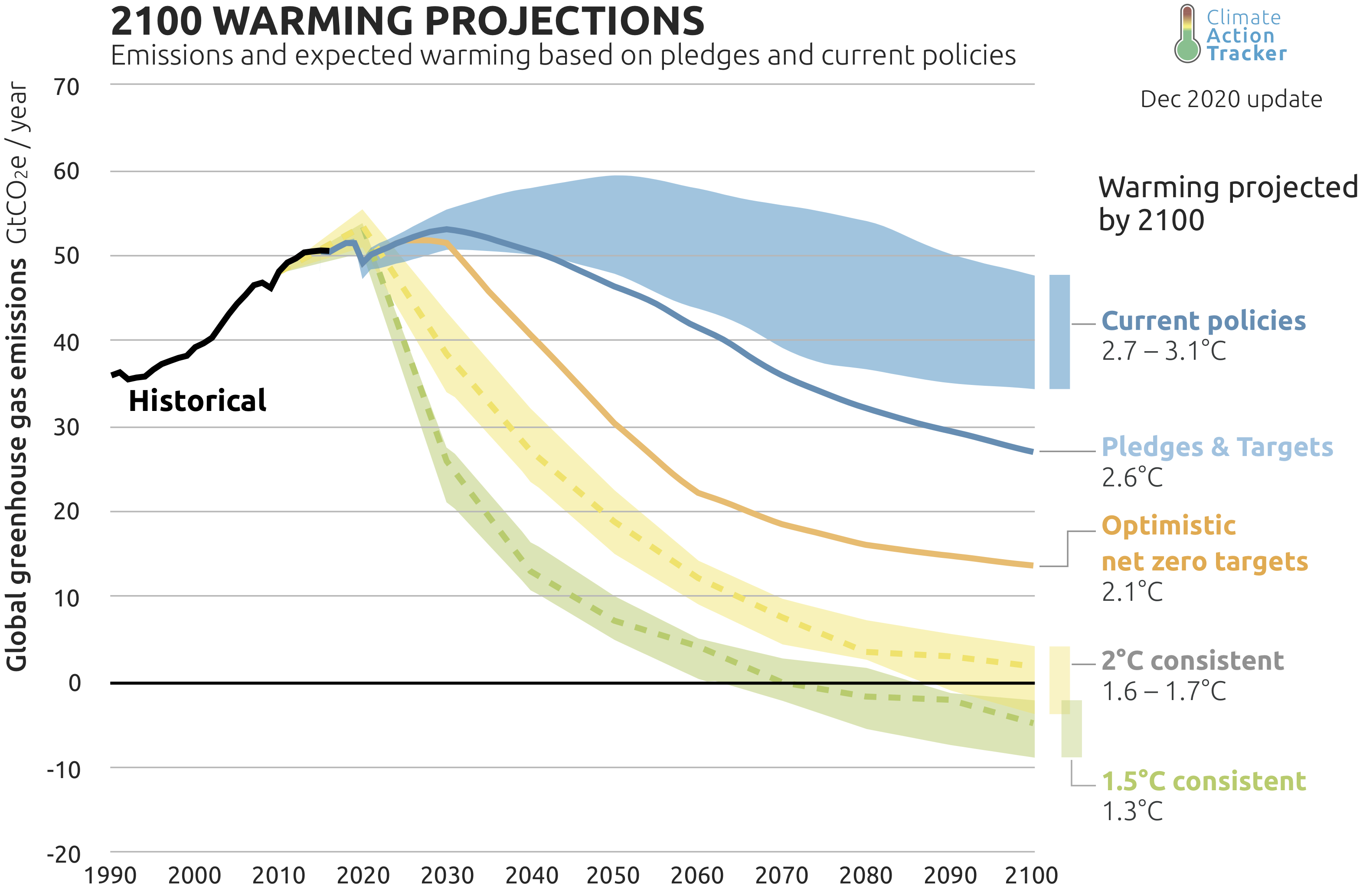
Pages 84, “our best guess”: Our “best guess” here roughly matches the IPCC scenario known as SSP3-7.0 scenario, leading to a 4°C temperature increase (see AR6 Figure TS.4 and AR6 Figure SPM.4), but it’s fair to say that there’s a lot of conventional wisdom at the moment behind a scenario more like SSP2-4.5, leading to 3°C. See my twitter thread here for more on why I’m not so optimistic, but in part it’s because I’m not convinced that countries can be trusted to meet their Paris Agreement pledges. For some other views, note that folks at Breakthrough think that world CO2 emissions peaked in 2019; the latest U.S. Energy Information Administration projection (IEO 2021) is that emissions in 2050 will be about 125% of 2019 emissions, with the rise continuing thereafter. See also International Energy Agency’s World Energy Outlook 2021, which notes that “every data point showing the speed of change in energy can be countered by another showing the stubbornness of the status quo.” As notes on pages 82-83, the key questions here are about economic growth (especially in poor countries that want to be the next China), about technological progress (especially with green technologies like wind, solar, and batteries), and about government policy. And, for those looking for much more optimistic scenarios, see AR6 Box 1.2, which concludes “that all emission pathways with no or limited overshoot of 1.5°C imply that global net anthropogenic CO2 emissions would need to decline by about 45% from 2010 levels by 2030, reaching net zero around 2050, together with deep reductions in other anthropogenic emissions, such as methane and black carbon. To limit global warming to below 2°C, CO2 emissions would have to decline by about 25% by 2030 and reach net zero around 2070.“

Page 84, “CO2 concentrations haven’t been that high for millions of years”: See AR6 Figure TS.1 and Kiehl 2011 (“Lessons from Earth’s Past”, ungated version may be here), which notes: “When was the last time the atmosphere contained ~1000 ppmv of CO2? Recent reconstructions of atmospheric CO2 concentrations through history indicate that it has been ~30 to 100 million years since this concentration existed in the atmosphere.”

Page 85, “about 4°C”: See AR6 Figure SPM.4 and AR6 Figure SPM.8.

Page 86, “the average summer in 2100”: See Battisti and Naylor 2009, “Historical warnings of future food insecurity with unprecedented seasonal heat”, Science 323:240-244.

Page 88, oceans, land areas, Arctic: See the projections for SSP3-7.0 in AR6 Table 4.2 and the accompanying text in AR6 Chapter 4.3.1.1: “Consistent with AR5, and earlier assessments, CMIP6 models project that annual average surface air temperature will warm about 50% more over land than over the ocean, and that the Arctic will warm about more than 2.5 times the global average.”

For ice-free Arctic, see AR6 TS.2.5: “The Arctic Ocean is projected to become practically sea ice-free in late summer under high CO2 emissions scenarios by the end of the 21st century (high confidence).” See also AR6 Figure TS.8.

Chapter 8: Water (pages 91-102)

Page 92, water cycle: See USGS, “The Water Cycle”.

Page 92, water vapor: A climate scientist colleague notes: “if you can see it, it’s not water vapor—the visible ‘mist’ is made of liquid water droplets. But the steam coming out of the teapot is water vapor!”

Page 94, “extra energy…ends up in the oceans”: See AR6 FAQ 7.1: “Research has shown that the excess energy since the 1970s has mainly gone into warming the ocean (91%), followed by the warming of land (5%) and the melting ice sheets and glaciers (3%).” (Warming of the atmosphere makes up the remaining 1% or so; see also AR5 (2014) Section TS.2.3.)

Page 94, thermal expansion, 6 inches during 20th century: AR6 Chapter 9 says: “Global mean sea level (GMSL) rose faster in the 20th century than in any prior century over the last three millennia (high confidence), with a 0.20 [0.15–0.25] m rise over the period 1901 to 2018 (high confidence). GMSL rise has accelerated since the late 1960s, with an average rate of 2.3 [1.6–3.1] mm yr-1 over the period 1971–2018 increasing to 3.7 [3.2–4.2] mm yr-1 over the period 2006–2018 (high  confidence). New observation-based estimates published since SROCC lead to an assessed sea level rise over the period 1901 to 2018 that is consistent with the sum of individual components. While ocean thermal expansion (38%) and mass loss from glaciers (41%) dominate the total change from 1901 to 2018, ice sheet mass loss has increased and accounts for about 35% of the sea level increase during the period 2006–2018 (high confidence).”

Page 95, “accelerating”: From above, GMSL rise was about 3.7 x 12 = 44.4mm over 2006-2018, about 2.3 x 47=108.1mm over 1971-2018, and about 200mm over 1901-2018, with an average rate of 3.7mm/yr over 2006-2018 (i.e., an inch every 7 years). We can calculate average rates for 1901-1971 as (200 – 108.1)/70 = 1.31mm/yr (i.e., an inch every 20 years). See also AR6 Figure 2.28. Need to update after final publication per draft corrigenda; check Executive Summary for this information.

Page 95, “2 feet of sea level rise”: See AR6 SPM.8, noting that 2 feet is about 0.6m.

Page 96, sea level rise and floating Arctic ice: To a first approximation, the melting of floating ice will not raise see levels. But melting Arctic ice will (modestly) contribute to sea level rise because of salinity differences between ice and ocean water. See Noerdlinger and Brower 2007, “The melting of floating ice raises the ocean level”, Geophysical Journal International 170:145-150, also discussed in NSIDC 2005.

Page 96, “Arctic Circle”: The quote comparing the Arctic to the Mediterranean is from Scott Borgerson, “The Coming Arctic Boom”, Foreign Affairs (July/Aug 2013).

Page 97, Winter Olympics: See The Future of the Winter Olympics in a Warmer World, described in the article “Climate change threatens Winter Olympics”. See also “The End of Snow?” by Powder magazine editor Porter Fox (NY Times, Feb 7 2014).

Page 97, snow: See AR6 SPM A.1.5: “Human influence very likely contributed to the decrease in Northern Hemisphere spring snow cover since 1950.” And also AR6 SPM B.3.1: “There is high confidence in an earlier onset of spring snowmelt, with higher peak flows at the expense of summer flows in snow-dominated regions globally.”

Page 98, “Clausius-Clapeyron”: See AR6 FAQ 8.2: “The heavy and sustained rainfall events responsible for most inland flooding are becoming more intense in many areas as the climate warms because air near Earth’s surface can carry around 7% more water in its gas phase (vapour) for each 1°C of warming. This extra moisture is drawn into weather systems, fueling heavier rainfall.” See also AR4 (2007) FAQ 3.2. A climate scientist colleague notes: “A good example of Clausius-Clapeyron in action is the fact that summer is much more humid than winter everywhere (even in Seattle, where it never rains in summer and always rains in winter!).”

Page 99, precipitation: See AR6 SPM A.3.2: “The frequency and intensity of heavy precipitation events have increased since the 1950s over most land area for which observational data are sufficient for trend analysis (high confidence), and human-induced climate change is likely the main driver. Human-induced climate change has contributed to increases in agricultural and ecological droughts in some regions due to increased land evapotranspiration (medium confidence).” Also AR6 SPM B.3.2: “A warmer climate will intensify very wet and very dry weather and climate events and seasons, with implications for flooding or drought (high confidence), but the location and frequency of these events depend on projected changes in regional atmospheric circulation, including monsoons and mid-latitude storm tracks.” See also AR5 (2014) FAQ 12.2: “These changes produce two seemingly contradictory effects: more intense downpours, leading to more floods, yet longer dry periods between rain events, leading to more drought.” See also AR5 (2014) Chapter 11.3.2.3.1: “The general pattern of wet-get-wetter… and dry-get-drier has been confirmed”.

Page 100-102, ocean acidification: AR6 Chapter 5 estimates 23% going into the oceans. It also says: “Ocean acidification is strengthening as a result of the ocean continuing to take up CO2 from human-caused emissions (very high confidence). This CO2 uptake is driving changes in seawater chemistry that result in the decrease of pH and associated reductions in the saturation state of calcium carbonate, which is a constituent of skeletons or shells of a variety of marine organisms.” See also AR5 (2014) Chapter 1.3.4.2: “[O]cean acidification poses potentially serious threats to the health of the world ocean ecosystems (see AR5 WGII assessment).” And here’s a neat video (including a do-it-yourself experiment!) from the University of Washington Dept of Atmospheric Sciences; there’s also an Australian video on Hermie the hermit crab. For the pH of Coca-Cola see ADA. A climate scientist colleague writes that ocean acidification is also connected with ocean warming: “Perhaps [in a future edition there will be] an opportunity to discuss the direct role of warming on marine ecosystems, which is at least as large a threat as ocean acidification…  [A]s the oceans warm, the metabolic rates of many marine species increase, meaning they need more oxygen, even while warmer water holds less oxygen – a double whammy that has led to extinction at very high warming levels in Earth’s history (e.g., see work of Penn et al. 2018 [“Temperature-dependent hypoxia explains biogeography and severity of end-Permian marine mass extinction“, Science 362(6419)].)”

Page 101, “tiny sea creatures”: See also stories in the media such as Craig Welch, “Sea changes harming ocean now could someday undermine marine food chain”, Seattle Times, Nov 25 2012. See also the Sixth Status of Corals of the World: 2020 Report, as described in Catrin Einhorn, “Climate Change Is Devastating Coral Reefs Worldwide, Major Report Says” (NY Times, Oct 4 2021).

Chapter 9: Life on Earth (pages 103-112)

Page 105, “caused by humans”: Note that the original five boxes connect to the acronym HIPPO: Habitat Loss, Invasive Species, Pollution, Human Population, and Overharvesting.

Page 105, “40-70% of species”: See AR4 (2007) Synthesis Report SPM: “As global average temperature increase exceeds about 3.5°C, model projections suggest significant extinctions (40-70% of species assessed) around the globe”. It doesn’t look like more recent reports try to quantify it, but AR5 (2014) Working Group II SPM says “substantial species extinction” with a 4°C temperature increase.

Chapter 10: Beyond 2100 (pages 113-124)

Page 115, “temperatures would stay high, and sea level would continue to rise, for hundreds of years”: AR6 Chapter 4 says: “Earth system modelling experiments since AR5 confirm that the zero CO2 emissions commitment (the additional rise in GSAT after all CO2 emissions cease) is small (likely less than 0.3°C in magnitude) on decadal time scales, but that it may be positive or negative. There is low confidence in the sign of the zero CO2 emissions commitment. Consistent with SR1.5, the central estimate is taken as zero for assessments of remaining carbon budgets for global warming levels of 1.5°C or 2°C.” But AR6 Figure 4.40(b) shows that temperatures continue to be elevated through 2300 even under scenarios, like SSP1-1.9, that have zero or negative CO2 emissions after 2050. (See AR6 SPM Box SPM.1 for details about the scenarios.) And AR6 Chapter 9 says: “Beyond 2100, GMSL will continue to rise for centuries due to continuing deep ocean heat uptake and mass loss of the Greenland and Antarctic Ice Sheets, and will remain elevated for thousands of years (high confidence).” PS. See also the figures about climate sensitivity in Roe and Bauman 2013.

Page 116, “CO2 is a long-lived gas”: There’s not much about this in IPCC AR6, but see AR5 (2014) FAQ 12.3: “For an emission pulse of about 1000 PgC, about half is removed within a few decades, but the remaining fraction stays in the atmosphere for much longer. About 15 to 40% of the CO2 pulse is still in the atmosphere after 1000 years.” See also AR5 (2014) Box 6.1, Figure 1. Note that the left and middle panels refer to an instantaneous CO2 pulse of 100 PgC; from the bottom of AR5 (2014) Figure TS.19 we see that fossil fuel emissions from the 1860s through 2005 have totaled about 300PgC. See also AR5 (2014) FAQ 6.2 and Archer and Brovkin 2008 (“The millennial atmospheric lifetime of anthropogenic CO2”, Climatic Change): “The largest fraction of the CO2 recovery will take place on time scales of centuries, as CO2 invades the ocean, but a significant fraction of the fossil fuel CO2, ranging in published models in the literature from 20-60%, remains airborne for a thousand years or longer. Ultimate recovery takes place on time scales of hundreds of thousands of years, a geologic longevity typically associated in public perceptions with nuclear waste.” Archer is also the author of the book The Long Thaw: How Humans Are Changing the Next 100,000 Years of Earth’s Climate (2010).

Page 118, “2 feet by 2100”: See AR6 SPM.8, noting that 2 feet is about 0.6m.

Page 119, Greenland: See AR6 FAQ 9.1: “For ice sheets that are mostly resting on bedrock above sea level – like the Greenland ice sheet – the main self-reinforcing loop that affects them is the ‘elevation–mass balance feedback’.” Also AR6 Box TS.9: “At sustained warming levels between 3°C and 5°C, near-complete loss of the Greenland Ice Sheet and complete loss of the West Antarctic Ice Sheet is projected to occur irreversibly over multiple millennia (medium confidence)…” AR6 Figure 9.2 shows that melting Greenland would be 7m [23 feet] of sea level rise.

Page 120, Antarctica: AR6 Figure 9.2 shows that melting the Antarctic Ice Sheet would be 58m [190 feet] of sea level rise. See also AR6 Box TS.4: “Importantly, likely range projections do not include those ice-sheet-related processes whose quantification is highly uncertain or that are characterized by deep uncertainty. Higher amounts of GMSL rise before 2100 could be caused by earlier-than-projected disintegration of marine ice shelves, the abrupt, widespread onset of Marine Ice Sheet Instability (MISI) and Marine Ice Cliff Instability (MICI) around Antarctica, and faster- than-projected changes in the surface mass balance and dynamical ice loss from Greenland (Box TS.4, Figure 1). In a low-likelihood, high-impact storyline and a high CO2 emissions scenario, such processes could in combination contribute more than one additional meter of sea level rise by 2100.“

Page 121: Elevation above sea level is about 6 feet in Miami and  13 feet in Shanghai. AR6 SPM B.5.3. says “Global mean sea level rise above the likely range—approaching 2 m [6.6 ft] by 2100 and 5 m [16.4 ft] by 2150 under a very high GHG emissions scenario (SSP5-8.5) (low confidence)—cannot be ruled out due to deep uncertainty in ice sheet processes.” And then AR6 Figure SPM.8 has a graphic about sea level rise in 2300 that says “Sea level rise greater than 15m [49 ft] cannot be ruled out with high emissions”.

Page 122, “The world population could be 2 billion… or 36 billion”: See the UN’s World Population in 2300 (2003), which has a best guess of world population in 2300 of 9 billion, with 2.3 billion as a low variant and 36.4 billion as a high variant.

Page 122, “imagine someone in 1900 trying to anticipate today’s world”: This idea is based on a fabulous article (actually a 1992 American Economic Association presidential address) by a Nobel Prize-winning economist: Schelling 1992, “Some economics of global warming”, American Economic Review 82:1-14.

Page 123, Arrhenius: See page 63 of his book Worlds in the Making: The Evolution of the Universe (1908): “We often hear lamentations that the coal stored up in the earth is wasted by the present generation without any thought of the future, and we are terrified by the awful destruction of life and property which has followed the volcanic eruptions of our days. We may find a kind of consolation in the consideration that here, as in every other case, there is good mixed with the evil. By the influence of the increasing percentage of carbonic acid in the atmosphere, we may hope to enjoy ages with more equable and better climates, especially as regards the colder regions of the earth, ages when the earth will bring forth much more abundant crops than at present, for the benefit of rapidly propagating mankind.”

Page 123, it’s tough to make predictions, especially about the future: This quote and variants of it are attributed to everyone from Mark Twain to Neils Bohr to Samuel Goldwyn, e.g., see The Economist. More from Quote Investigator, which concludes that it’s probably Danish in origin.

Chapter 11: Uncertainty (pages 125-136)

Page 127, “these odds are less than 1 in 3”: For probability terminology, see AR6 SPM footnote 4. For it being “exceptionally unlikely” that Greenland will melt in the 21st century, see AR5 (2014) Table 12.4. Regarding the lottery, the odds of winning Powerball are apparently about 1 in 175 million.

Page 128, “scientific predictions”: On temperatures, see AR6 Figure 1.9 and AR5 (2014) Figure 1.4. On sea level rise, see AR5 (2014) Figure 1.10. On both temperature and sea level rise, see also AR6 TS.1.2.2: “Projections of the increase in global surface temperature, the pattern of warming, and global mean sea level rise from previous IPCC Assessment Reports and other studies are broadly consistent with subsequent observations.”

On methane, see AR5 (2014) Figure 1.6. For more recent data, see AR6 Figure 2.5, and note that AR6 TS2.2 says: “In the 1990s, CH4 [methane] concentrations plateaued, but started to increase again around 2007 at an average rate of 7.6 ± 2.7 ppb yr-1 (2010–2019; high confidence). There is high confidence that this recent growth is largely driven by emissions from fossil fuel exploitation, livestock, and waste.”

On Arctic ice, see AR5 (2014) Chapter 1.3.4.3, which says “Sea ice extent has been diminishing significantly faster than projected by most of the AR4 climate models.” (See also the graphic in this Arctic Sea Ice Blog post and AR5 (2014) Chapter 4.8.) In the most recent report, AR6 TS.1.2.2 says that “[the more recent] CMIP6 models better simulate the sensitivity of Arctic sea ice area to anthropogenic CO2 emissions, and thus better capture the time evolution of the satellite-observed Arctic sea ice loss (high confidence).”

Page 130, “don’t put the microphone in front of the speaker”: This is a reference to Roe and Baker 2007 (“Why Is Climate Sensitivity So Unpredictable?” Science); they argue that feedbacks make it harder to rule out high climate sensitivities than low climate sensitivities.

Page 130, “negative feedback loop”: See AR5 (2014) Section 1.2.2: “The dominant negative feedback is the increased emission of energy through LWR [longwave radiation] as surface temperature increases (sometimes also referred to as blackbody radiation feedback).”

Page 133, “if reality turns out to be worse than we’d thought”: See for example AR6 FAQ5.2: “Can thawing permafrost substantially increase global warming?” or AR5 (2014) FAQ 6.1: “Could Rapid Release of Methane and Carbon Dioxide from Thawing Permafrost or Ocean Warming Substantially Increase Warming?”

Page 136, insurance: The “insurance” metaphor/argument is found repeatedly in economics discussions of climate change, e.g., Marty Weitzman: “The basic issue here is that spending money to slow global warming should perhaps not be conceptualized primarily as being about consumption smoothing as much as being about how much insurance to buy to offset the small change of a ruinous catastrophe that is difficult to compensate by ordinary savings” (Weitzman 2007, “A Review of The Stern Review on the Economics of Climate Change“, Journal of Economic Literature 45:703-724).

Chapter 12: The Tragedy of the Commons (pages 139-148)

Page 141, costs and benefits: See for example Cass Sunstein, “Climate Change: Lessons From Ronald Reagan” (NY Times, Nov 10 2012): “Economists of diverse viewpoints concur that if the international community entered into a sensible agreement to reduce greenhouse gas emissions, the economic benefits would greatly outweigh the costs.” One prominent cost-benefit model is the Yale economist Bill Nordhaus’s DICE model; see here. A related concept is the “social cost of carbon”, which estimates the optimal carbon tax for dealing with climate change; see this EPA analysis.

Page 142, tragedy of the commons: “The tragedy of the commons” (easier to read in PDF) refers to a 1968 article in Science by Garrett Hardin. For more on this see our Cartoon Econ books, especially Volume One: Microeconomics.

Page 143, Aristotle: See Aristotle’s Politics (written 350 B.C.E., translated by Benjamin Jowett), Book Two, Part III: “For that which is common to the greatest number has the least care bestowed upon it. Every one thinks chiefly of his own, hardly at all of the common interest; and only when he is himself concerned as an individual.”

Page 145, entire countries: The reference here is to efforts like the Kyoto Protocol, an attempted global CO2 treaty from the 1990s. As noted by Wikipedia, “The U.S. signed the Protocol, but did not ratify it [and] the U.S. Senate passed the Byrd-Hagel Resolution unanimously disapproving of any international agreement that 1) did not require developing countries to make emission reductions and 2) “would seriously harm the economy of the United States”. In addition, Wikipedia notes that “In 2011, Canada, Japan and Russia stated that they would not take on further Kyoto targets. The Canadian government announced its withdrawal [from] the Kyoto Protocol on 12 December 2011… Canada was committed to cutting its greenhouse emissions to 6% below 1990 levels by 2012, but in 2009 emissions were 17% higher than in 1990.” Finally, it’s worth noting that developing countries like China and India had no binding emissions targets under the Kyoto Protocol.

Page 146, “self-interest is not all bad”: Adam Smith was a Scottish philosopher and “the father of modern economics”. The quote about the butcher, the brewer, and the baker comes from The Wealth of Nations, first published in 1776. (You can still buy it today, and though not always a page-turner it’s remarkably readable.)

Page 146, “sometimes self-interest happens to coincide with emissions reductions”: These are called “co-benefits”, many of them dealing with the health benefits of reduced (local) air pollution that can accompany reductions of (global) CO2 emissions. See for example here, here, and here.

Page 147, “history shows that”: See for example “The Montreal Protocol, a Little Treaty That Could” (NY Times, Dec 9 2013).

Page 148, border tax adjustments: See for example Brad Plumer, “Europe Is Proposing a Border Carbon Tax. What Is It and How Will It Work?” (NY Times, July 14 2021). There are plenty of questions about BTAs, both legal questions (e.g., about whether BTAs would violate international trade rules) and economic/policy questions (e.g., how would you actually try to calculate the carbon content embedded in a computer made in Taiwan?). For one perspective here see the Carbon Tax Center.

Chapter 13: Techo-Fix (pages 149-162)

Page 150, geoengineering: See for example the Oxford Geoengineering Program. An early-ish article about this was “How Earth-Scale Engineering Can Save the Planet” (Popular Science, June 22 2005).

Page 150, “genetically modified carbon-eating trees”: The reference is to an article about physicist Freeman Dyson (“The Civil Heretic”, NY Times, Mar 25 2009):

Then he added the caveat that if CO2 levels soared too high, they could be soothed by the mass cultivation of specially bred “carbon-eating trees,” whereupon the University of Chicago law professor Eric Posner looked through the thick grove of honorary degrees Dyson has been awarded—there are 21 from universities like Georgetown, Princeton and Oxford—and suggested that “perhaps trees can also be designed so that they can give directions to lost hikers.”

Page 151, “the single best objection to the garden hose idea”: The quote is from Super Freakonomics, a 2009 book by University of Chicago economist Steven Levitt and journalism Stephen Dubner. The chapter on climate change in the book prompted a strong response from climate scientists, including Levitt’s U of C colleague Ray Pierrehumbert’s quite amusing blog post “An open letter to Steve Levitt”. My own thoughts on the book, and my email exchange with Levitt, is on my blog: Part 1, Part 2, Part 3.

Page 155, “negawatts”: The term “negawatts” was coined by Amory Lovins of the Rocky Mountain Institute.

Page 157, subsidies: The International Energy Agency said that global fossil fuel subsidies in 2020 were $180 billion, down 40% from 2019 levels. Because 2020 was such a strange year we’re using the 2019 value, namely $180b/0.6 = $300 billion. FYI the IEA estimate for 2010 was $409 billion.

Page 162, controversy: See for example Roger Pielke Jr’s “Iron Law” of Climate Policy.

Chapter 14: Putting a Price on Carbon (pages 163-174)

This material can all be found in any introductory environmental economics textbook, and a good bit of it is in our Cartoon Econ books.

Page 166, B.C. carbon tax: More from my 2012 NY Times op-ed (“The Most Sensible Tax of All”, co-authored with Shi-Ling Hsu), Sustainable Prosperity’s 2013 report on BC’s Carbon Tax Shift After Five Years, and lots from Sightline Institute’s blog, e.g., this.

Page 170, fisheries: Cap and trade systems for fisheries are usually called catch share systems or IFQ or ITQ systems (“individual fishing quota” or “individual transferable quoata”). The USA has a number of such policies; for details see NOAA. Note that such policies often feature multi-year permits, e.g., if you have a 1% catch share and the Total Allowable Catch is 100,000 tons this year and 150,000 tons next year then you get to catch 1,000 tons this year and 1,500 tons next year.

Page 174, “a necessary and sufficient step”: The quote is from Yale economist William Nordhaus, winner of the 2018 Nobel Prize in Economics, who wrote in 2008 that “To a first approximation, raising the price of carbon is a necessary and sufficient step for tackling global warming. The rest is at best rhetoric and may actually be harmful in inducing economic inefficiencies” (A Question of Balance: Weighing the Options on Global Warming Policies, 2008, full text available here).

Chapter 15: Beyond Fossil Fuels (pages 175-186)

Page 176, CH4 and CF4: See AR6 Table 7.SM.7 (in the supplement to Chapter 7), which shows that methane (CH4) has a 100-year GWP of 27.9 and CF4 has a 100-year GWP of 7,380. Note that CO2 is the benchmark used to discuss the Global Warming Potential (GWP) of other greenhouse gases. (The GWP of CO2 is always defined to be 1, with other gases measured in terms of their CO2 equivalents.) The topic is a bit tricky because all of these gases have varying atmospheric lifetimes, and as a result GWPs are defined for a given time frame, e.g., over 20 years methane (CH4) has a GWP of 81 (meaning that over 20 years a tonne of methane generates as much warming as 81 tonnes of CO2) but over 100 years methane has a GWP of only 28; that’s because CO2 is a long-lived gas and methane is not.

Page 179, rich countries, poor countries: See FAO’s FAO, Global Forest Resources Assessment 2020, Tables 7 and 8. See also Global Forest Resources Assessment 2010, which says that “around 13 million hectares of forests were converted to other uses or lost through natural causes each year in the last decade” but that the net change in forest area is only – 5.2m hectares per year. It also says that China is afforesting rapidly. On Norway and Indonesia, see here and here and here.

Page 181, methane feedback: See AR6 FAQ 5.2: “Can thawing permafrost substantially increase global warming?” The answer:  Projections suggest that “future permafrost thaw will lead to some additional warming – enough to be important, but not enough to lead to a ‘runaway warming’ situation, where permafrost thaw leads to a dramatic, self-reinforcing acceleration of global warming.”

Page 182, CF4 and black carbon:  On CF4, see AR6 Table 7.SM.7 (in the supplement to Chapter 7), which says that it has a 100-year GWP of 7,380 and a lifetime of 50,000 years. On black carbon, see AR6 Table 6.1, which says that black carbon (BC) has a lifetime of “minutes to weeks”, and AR6 FAQ 6.1, which says that black carbon remains in the atmosphere for days.

Page 183, “big three”: AR6 Figure 7.8 attributes temperature changes primarily to CO2 and methane, and CO2 from deforestation makes up about 10-20% of total anthropogenic CO2 emissions (see p46).

Page 184, “offsets are also used in many cap and trade systems”: For a skeptical view of this practice, see Cullenward and Victor, Making Climate Policy Work (2020) or Annie Leonard’s video “The Story of Cap & Trade” (2009).

Chapter 16: The Challenge (pages 187-200)

Page 191, “without proper maintenance”: See this Cornell University page on Compost Physics: “Compost managers strive to keep the compost below about 65°C because hotter temperatures cause the beneficial microbes to die off.”

Page 194, “our task is daunting”: This is a version of the IPAT equation; see also the related Kaya Identity.

Page 195, “remember that CO2 stays in the atmosphere for a long, long time”: See page 114 and the associated notes and references there.

Page 197, “it’s okay if your dream is different”: An “all-out mobilization” is a reference to the ideas of Joseph Romm of ClimateProgress.org; see his 2006 book Hell and High Water: Global Warming–the Solution and the Politics–and What We Should Do, excerpted here. The “breakthrough” panel references the ideas of the Breakthrough Institute.

Page 199, “join a chorus”: More here on the Energy & Enterprise Initiative, which aims to “put the works on climate change from a right-of-center market-friendly angle focused on revenue-neutral carbon taxes; on the Sierra Club; and on Citizens Climate Lobby, a grassroots group working for federal “fee and dividend” legislation.

Glossary (pages 201-209)

Air: See the entry for “atmosphere” in the AR6 Glossary for contents of the atmosphere. Note that the percentages are for dry air, but water vapor only averages 1% of the total.

Albedo: See the entry for “energy budget” in the AR6 Glossary for Earth’s 30% albedo.

Ice ages: See the entry for “glacial” in the AR6 Glossary; it says that the Last Glacial Maximum peaked about 21,000 years ago.

Interglacial period: See the entry for “interglacial” in the AR6 Glossary; it says that the  current interglacial period, called the Holocene, started about 12,000 years ago.

Marine Ice Cliff Instability and Marine Ice Sheet Instability: See the entries for these in the AR6 Glossary; note in particular this about MICI: “If the exposed ice cliff is tall enough (about 800 m of the total height, or about 100 m of the above-water part), the stresses at the cliff face exceed the strength of the ice, and the cliff fails structurally in repeated calving events.” See AR6 FAQ 9.1 about MISI. Also AR6 Box TS.4.

Temperature: See the entry for “energy budget” in the AR5 (2014) Glossary for current global average temperature of 15°C.

PS. Potential improvements for 3rd edition (and release notes)

• Tell Kickstarter supporters
• Work with IP on page notes webpage
• p8: No …s after N1 or before N2?
• p29: “past 10,000 years”: is there a better way to show this? Maybe with thumb and 2nd finger indicating size?
• p79: Add nuclear?
• p80 and p140: Edit to “rest of developing Asia”?
• p116: Debold “what we meant”?
• p178: Add something about burning or decomposition?